arrow_back Back home

4 November 2022

Paper notes: "Computation of Regions of Attraction for Hybrid Limit Cycles Using Reachability"

These are my notes from the below paper.

Jason J. Choi, Ayush Agrawal, Koushil Sreenath, Claire J. Tomlin, and Somil Bansal

IEEE Robotics and Automation Letters (RA-L), and International Conference on Robotics and Automation (ICRA), 2022 [PDF] [Code and Videos]

Abstract

Contact-rich robots (with legs or manipulators) are often represented as hybrid systems (due to the discontinuous state changes upon contact, state resets).
These state resets make modeling the stability and region-of-attraction difficult.
In this work, the region-of-attraction is modeled as a Hamilton-Jacobi (HJ) reachability problem [1]. Further, the HJ reachability framework is generalized to handle the discontinuities of hybrid systems.
“The key idea of our new numerical method is very simple, which is that the two states before and after the reset always have the same value.”

I. Introduction

Legged robots are often represented as hybrid systems, where the swinging of the legs are continuous and contact events with the ground are discrete. Gaits are then defined as hybrid limit cycles (a limit cycle with discontinuous jumps).

For stable behavior, a region of attraction (RoA) is calculated– the configuration space from which the robot can return to the desired limit cycle (gait). This work casts the RoA computation as an HJ reachability problem, then they compute the backward reachable tube (BRT)– “the set of states such that the trajectories that start from this set will eventually reach some given target set despite the worst case disturbance.”

Although BRT computation is more expensive than existing methods, it can recover the full RoA without any restrictions on its shape.

To overcome state resets, they apply the Bellman principle of optimality at the switching surface.

Poincaré map-based methods

By JJ Harrison (https://www.jjharrison.com.au/) - Own work, CC BY-SA 3.0, https://commons.wikimedia.org/w/index.php?curid=16998146

Analyze the stability of a fixed point in the Poincaré map that corresponds to a given limit cycle. If this fixed point is stable, then there exists a stable limit cycle for the system that passes through it.

Downside: Finding an analytical solution (a mathematical expression) for a Poincaré map is challenging. The verifiable RoA is restricted to the configuration space of the chosen Poincaré section.

Lyapunov-based methods

Construct a time-varying Lyapunov function using a sum-of-squares (SOS) program.

Stabilizing controllers for hybrid systems with state resets

Hybrid zero dynamics (HZD) can create stabilizable hybrid limit cycles and stabilizing controllers for walking robots with discrete impacts. The Poincaré method can be added to HZD to create event-based controllers (which can stabilize or switch between limit cycles).

[2] proposes a rapidly exponentially stabilizing control Lyapunov function that can stabilize hybrid limit cycles. Other work has leveraged value mapping to account for state resets. This work extends value mapping to handle reachability and RoA computation as opposed to trajectory optimization.

III. Problem setup

Consider the following class of hybrid systems:

\[\begin{equation} \displaylines{ \dot{x} = f(x,u,d), x\notin S \\ x^+=\Delta(x^-), x^-\in S } \label{ref1}\tag{1}\end{equation}\]

where \(x\in \mathbb{R}^n\) is the state, \(u\in \mathcal{U}\) is the control input, \(S\) is the switching surface (the ground), and \(d \in \mathcal{D}\) is the disturbance. When a reset event occurs at time \(t\), the state \(x^-\) immediately shifts to \(x^+\).

In other words, the change in state when not in contact with the ground depends on the current state, the control input, and disturbances, and the function \(\Delta(\cdot)\) moves the state from \(x^-\rightarrow x^+\) when the state is in contact with the switching surface.

The result is a set of continuous trajectories along the vector flow \(f\), with jumps whenever the state touches \(S\).

Hybrid limit cycle

\(x^*(\cdot)\) is a hybrid limit cycle if it undergoes impacts periodically. The hybrid limit cycle is paired with a baseline control law \(\pi_0(\cdot):\mathbb{R}^n\rightarrow\mathcal{U}\) that makes the limit cycle forward invariant and stable in its immediate neighborhood.

Two-part objective:

Compute a state space \(\Omega(x^*)\subseteq \mathbb{R}^n\) in the region around the hybrid limit cycle \(x^*(\cdot)\) from which the system can asymptotically stabilize to \(x^*(\cdot)\). Then \(\Omega(x^*)\) is simply the region of attraction (RoA) w.r.t. the hybrid limit cycle.
Design the corresponding control law through which the system can stabilize to \(x^*\).

The work focuses on finding the maximal RoA– that is, the RoA that can be reached by the best-case controller, not just a given baseline controller.

Running example (Teleporting Dubins’ Car)

A Dubins path is the shortest curve that connects two points in the x-y plane under curvature constraints and given prescribed initial and terminal tangents. Under states R (right turn), L (left turn) and S (straight), the optimal path will always be either RSR, RSL, LSR, LSL, RLR, or LRL.

By Salix alba - Own work, CC BY-SA 4.0, https://commons.wikimedia.org/w/index.php?curid=46816719

Dubins’ cars have simple dynamics:

\[\begin{equation}\displaylines{ \dot{p}_x=v\cos\theta, \dot{p}_y=v\sin\theta, \dot{\theta}=u }\label{ref2}\tag{2}\end{equation}\]

Then state \(x=\{p_x,p_y,\theta\}\) and the input \(u\in\{-\bar\omega,\bar\omega\}\) is the angular speed. The switching surface and reset maps are then:

\[\begin{equation}\displaylines{ S=\{x|p_y=0,\sin\theta<0\} \\ x^+=\Delta(x^-)=[-R\cdot(|p_x|/R)^\alpha\cdot sign(p_x)] }\label{ref3}\tag{3}\end{equation}\]

where \(R\) is the radius of the desired semi-circular hybrid limit cycle. When \(\alpha=1, p^+_x=-p_x\) such that the car’s position is mirrored on the y axis. When

\(\alpha<1\),

the reset map causes the value of \(\|p_x\|\) to converge to \(R\). Finally, when \(\alpha>1\), the value of \(\|p_x\|\) expands away from \(R\).

We wish to attain a limit cycle with a semi-circular trajectory of radius \(R\) centered at the origin with a counterclockwise direction:

\[\begin{equation}\displaylines{ x^*(\cdot)=\{x\mid||(p_x,p_y)||=R, \theta=\frac{\pi}{2}+\arctan(\frac{p_y}{p_x}),\frac{\pi}{2}\le\theta<\frac{3\pi}{2}\} }\label{ref4}\tag{4}\end{equation}\]

Our goal is therefore to compute the region-of-attraction (RoA) for \(x^*(\cdot)\) – that is, the states from which the car can be stabilized to asymptotically converge to (\(\ref{ref4}\)). We therefore define a baseline stabilizing controller \(\pi_0(\cdot)\) designed by feedback linearization with output defined as \(y=\|(p_x,p_y)\|-R\).

IV. Background

A. Hamilton-Jacobi Reachability

Let \(\dot{x}=f(x,u)\) be the dynamics of a continuous system without disturbance, let \(\xi^u_{x,t}(\tau)\) denote the state achieved at time \(\tau\) by starting at initial state and time \({x,t}\) and by applying input functions \(u(\cdot)\) over \([t,\tau]\).

Given target set \(\mathcal{L}\subset\mathbb{R}^n\), we want to find the Backward Reachable Tube (BRT) of \(\mathcal{L}\). The BRT is the set of initial states from which the agent acting optimally will eventually reach \(\mathcal{L}\) within the time horizon \([t,\tau]\):

\[\begin{equation}\displaylines{ \mathcal{V}(t)=\{x\mid\exists u(\cdot):[t,T]\rightarrow\mathcal{U},\exists\tau\in[t,T],\xi^u_{x,t}(\tau)\in\mathcal{L}\} }\label{ref5}\tag{5}\end{equation}\]

In HJ reachability, BRT is an optimal control problem solved using dynamic programming.

We define Lipschitz continuous target function \(l(x)\) which is less than zero for each point in the target set: \(\mathcal{L}=\{x:l(x)\le0\}\). Typically, \(l(x)\) is the signed distance function to \(\mathcal{L}\).

The BRT finds all states that could enter \(\mathcal{L}\) at any point in the time horizon \([t,\tau]\). That is, given a state \(x\), initial time \(t\), and input function \(u(\cdot)\), we find the minimum distance to the target set within the horizon:

\[\begin{equation}\displaylines{ J(x,t,u(\cdot)=\min_{\tau\in[t,T]}l(\xi^u_{x,t}(\tau)) }\label{ref6}\tag{6}\end{equation}\]

The goal is to find (\(\ref{ref6}\)) for optimal trajectories of the system. This means that we compute the optimal control that eventually drives the system into the target set \(\mathcal{L}\) when \(l(\cdot)\le0\). The value function is then:

\[\begin{equation}\displaylines{ V(x,t)=\inf_{u(\cdot)}\left\{J(x,t,u(\cdot))\right\} }\label{ref7}\tag{7}\end{equation}\]

That is, given the state \(x\) and initial time \(t\), (\(\ref{ref7}\)) is the infimum of the minimum signed distance between the target set \(\mathcal{L}\) and the target function \(l(x)\) across all possible controls \(u(\cdot)\).

We can optimize the computation of (\(\ref{ref7}\)) using dynamic programming, which results in the Hamilton-Jacobi Isaacs Variational Inequality (HJI-VI):

\[\begin{equation}\displaylines{ \min\left\{ D_tV(x,t)+H(x,t),l(x)-V(x,t) \right\}=0 }\label{ref8}\tag{8}\end{equation}\]

with the resulting value function being \(V(x,T)=l(x)\). \(D_t, \Delta\) represent the time and spatial gradients of the value function. \(H\) is the Hamiltonian function that encodes the role of dynamics and optimal control inputs:

\[\begin{equation}\displaylines{ H(x,t)=\min_u\langle\Delta V(x,t), f(x,u)\rangle }\label{ref9}\tag{9}\end{equation}\]

That is, the Hamiltonian is the combined minimum of the gradient of the value function and \(f(x,u)\) across all control inputs \(u\). The optimal control for reaching target set \(\mathcal{L}\) is then:

\[\begin{equation}\displaylines{ u^*(x,t)=\arg \min_u\langle\Delta V(x,t),f(x,u)\rangle }\label{ref10}\tag{10}\end{equation}\]

B. Casting RoA computation as an HJ reachability problem

\[\begin{equation}\displaylines{ u(x,t) = \begin{cases} \arg \min_u\langle\Delta V(x,t),f(x,u)\rangle & \text{if } x \notin \mathcal{L}\\ \pi_0(x) & \text{otherwise} \end{cases} }\label{ref11}\tag{11}\end{equation}\]

(\(\ref{ref11}\)) is a stabilizaing controller than can be used to steer the system to \(\mathcal{L}\) from any state within the BRT and then switch to the baseline controller when \(x\in\mathcal{L}\).

For the teleporting Dubins’ car example, the target function is \(l(x):=\|(p_x,p_y)\|-R-\epsilon\).

C. Robustness to bounded disturbance

HJ reachability can design optimal controllers that are resistant to bounded disturbance \(d\in\mathcal{D}\). In this mode, the BRT is now the set of initial states \(x\) for which, under worst-case disturbances, the agent acting optimally will eventually reach the target set \(\mathcal{L}\) within the time horizon \([t,\tau]\):

\[\begin{equation}\displaylines{ \mathcal{V}(t)=\{x:\exists u(\cdot), \forall d(\cdot):[t,T]\rightarrow\mathcal{D},\exists\tau\in[t,T], \xi^{u,d}_{x,t}(\tau)\in\mathcal{L}\} }\label{ref112}\tag{12}\end{equation}\]

Computation of the BRT can be treated as a two-player, zero-sum game between P1 (the controller) and P2 (the disturbance). Let the Hamiltonian be:

\[\begin{equation}\displaylines{ H(x,t)=\max_u\min_d\langle\Delta V(x,t),f(x,u)\rangle }\label{ref13}\tag{13}\end{equation}\]

Finally, the optimal, disturbance-robust control signal is:

\[\begin{equation}\displaylines{ u^*(x,t) = \arg\max_u\min_d\langle\Delta V(x,t),f(x,u)\rangle }\label{ref14}\tag{14}\end{equation}\]

VI. Case studies

A. Running example: Teleporting Dubins’

Used Dubins’ car with contracting reset map (\(\alpha<0.5\)).

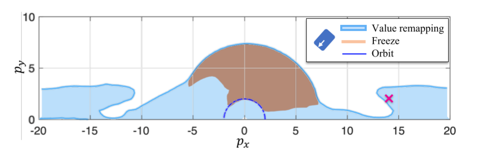
The blue region is the BRT where value remapping is applied, and the brown region is where frozen dynamics are applied. Both are given a time limit \(T=6.3 s\). Notice that the frozen dynamics BRT is always contained within the BRT of the proposed method– in other words, value remapping can produce a much larger BRT.

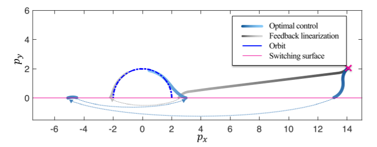
Here, the Dubins’ car is initialized at the cross with \(\theta=-3\pi/4\).

C. Compass-gait walker

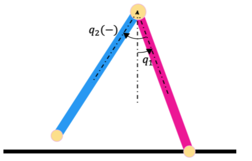
A compass-gait walker is a simple bipedal model composed of just two links. Walking is treated as a hybrid model, where the gait is separated into:

a continuous single-support phase (one contact) and
an instantaneous, inelastic impact (two contacts)

The continuous dynamics are then modeled as a control-affine: \(\dot{x}=f(x)+g(x)u\), and the switching surface is:

\[\begin{equation}\displaylines{ S:=\{x\mid q_1\le \bar{q_1}, 2q_1 + q_2=0, 2\dot{q_1}+\dot{q_2}<0 \} }\label{ref15}\tag{15}\end{equation}\]

where \(q=[q_1,q_2]^T\) is the walker’s configuration variable.

The BRTs are evaluated first with the baseline controller and then with the optimal controller under control bound \(u\in[-4,4]N\). It’s determined that the proposed method produces a much larger, maximal BRT versus the limited BRT of the baseline controller.

Finally, disturbances are introduced in the form of a stiction torque on the single joint: \(\dot{x}=f(x)+g(x)u+\dot{q_2}g(x)d\). This disturbance accounts for any unmodeled disturbances in the system. It is determined that the the system can still robustly stabilize the walker under disturbance, and that it produces a larger RoA than the CLF-QP does.

VII. Conclusion and future work

The authors find that their method, which expands HJ reachability to handle hybrid systems with state resets, was able to produce larger regions of attraction than the state-of-the-art approaches. Their method simultaneously produces a controller that can robustly stabilize against disturbances (such as unmodeled dynamics).

Limitation: Reachability scales exponentially with the number of states. This could possibly be mitigated using neural net-based PDE solvers.

Glossary

Dynamic Programming

Dynamic programming refers to the simplification of a complicated problem by breaking it down into smaller problems recursively. Decisions that span across time are often capable of being optimized in this way. The relationship between the value of the large problem and the values within the smaller problems is called the Bellman equation.

Feedback linearization

A technique applied to nonlinear control systems that transforms it into a fully or partially decoupled linear system using a change of variables and a suitable control input. This allows linear control strategies to be used.

Generally, we select a nonlinear transformation \(z=T(x)\) and a nonlinear state feedback variable \(v=\alpha(x)+\beta(x)u\) [3].

Forward invariance

As Chai and Sanfelice put it, “A forward invariant set for a dynamical system is a set that has solutions evolving within the set… it characterizes regions of the state space from which solutions start and stay for all future time.”

Hamiltonian

Inspired by Hamiltonian mechanics and developed by Lev Pontryagin as part of his maximum principle.

A necessary condition for solving an optimal control problem is that the chosen control should optimize the Hamiltonian.

Consider a dynamical system of first-order DEs:

\[\dot{\bf x}(t)={\bf f}({\bf x}(t),{\bf u}(t),t)\]

where (\({\bf x, u}\)) are vectors of states and controls. In optimal control, we must choose \(\bf u\) such that \(\bf x\) maximizes an objective function in the interval \([t,\tau]\). This involves defined the control Hamiltonian:

\[H({\bf x}(t),{\bf u}(t),{\bf \lambda}(t),t)\equiv I({\bf x}(t),{\bf u}(t),t)+\lambda^T(t){\bf f}({\bf x}(t), {\bf u}(t), t)\]

where \(I(\cdot)\) gives the performance index at each point in time and the multipliers \(\lambda(t)\), referred to as costate variables, are functions of time.

Goal: Find an optimal control policy \({\bf u}^*(t)\) and with it an optimal trajectory \({\bf x}^*(t)\), which under Pontryagin’s maximum principle must maximize \(H\) (above). Specifically:

\[H({\bf x^*}(t),{\bf u^*}(t),{\bf \lambda}(t),t) \ge H({\bf x}(t),{\bf u}(t),{\bf \lambda}(t),t)\]

for all \({\bf u}(t)\in \mathcal{U}\).

Hybrid system

A system with both continuous and discrete-time behavior. Can both “flow” (with differential EQ) and “jump” (e.g. state machine) [4].

Hybrid systems are useful due to their flexibility and ability to incorporate many kinds of subsystems. The state of a hybrid system is usually defined by the values of its continuous variables and a discrete mode.

A classic example of a hybrid system is a bouncing ball, which has a continuous state when above the ground yet discrete/instantaneous when it hits the ground.

Infimum and supremum

Given a set \(S\) and subset \(P\):

The infimum \(\inf(P)\) is the greatest element in \(S\) that is less than or equal to each element in \(P\).
The supremum \(\sup(P)\) is the least element in \(S\) that is greater than or equal to each element in \(P\).

Inf. and sup. have many useful applications in set theory. They are close to but not the same as min and max. For example, the infimum of positive real numbers \(\mathbb{R}^+\) relative to all real numbers \(\mathbb{R}\) is zero, since zero is the greatest element in \(\mathbb{R}\) that is less than or equal to any positive number.

Lipschitz continuous function

A function with a strong form of continuity where a double cone can be moved along the graph without the function ever entering the cone.

Taschee, CC0, via Wikimedia Commons

Lyapunov function

Scalar functions used to determine the stability of an equilibrium within a given ODE.

Reachable tube

Unlike a reachable set, which is the set of possible states exactly at time 0, a reachable tube is the set of all states that can be reached within the time horizon. Useful for safety analysis, since we wish to determine if the system can reach an unsafe state ever within the horizon.

Sum-of-squares (SOS) programming

As Wang Yimu writes, SOS programs ask if a polynomial function \(f\) can be factored as the sum of squares of polynomial basis \(b\). Example:

\[f=(1,x, x^2, x^3)\Rightarrow ||f||^2=1+x^2+x^4+x^6\]

If an SOS exists for \(f\), then \(f(x)>0\) for all \(x\).

Value function

Value functions provide the value of the objective function (e.g. cost function) at a solution while only depending on the system’s parameters. In a controlled dynamical system, it represents the optimal payoff over \([t,\tau]\).

The value function can be thought of as the cost to finish the optimal program, the “cost-to-go function.” (Wikipedia)

Zero-shot learning

A form of machine learning where at test time the model classifies observations into categories that it wasn’t trained on. This is in contrast to the more basic approach, where the training and testing sets include examples from the exact same classes.