arrow_back Back home

29 October 2022

Zonotopes!

Introduction

Zonotopes are a class of sets that have some special properties. Here, I’ll explain what zonotopes are, along with their related classes. I’ll explain their use in state estimation and optimization in a future article.

Standard zonotopes are a subset of constrained zonotopes, which are a subset of hybrid zonotopes, which are a subset of convex polytopes… Got that?

Due to common math rendering issues online, I would recommend viewing this article as a PDF.

Convex polytopes

(Wikipedia)

A polytope is the n-dimensional generalization of a polygon (2D) or polyhedron (3D). Polytopes can help us represent sets. Imagine a set of datapoints in three dimensions, spread out into a cloud. It’s easier to represent this vague cloud of data in a neat box. A properly-sized polytope can serve as the perfect box.

It turns out that convex polytopes are extra-special boxes, as they can be extended further into zonotopes.

Before talking about that, how can convex polytopes be represented? In other words, if you’re telling your friend about the box you found, how would you describe it?

Vertex representation (convex hull)

A set \(K\) is convex if, for any pair of points \(a,b\in K\), the segment between them is contained within \(K\). We can define a convex polytope as the convex hull of a finite set of points, and therefore describe the convex polytope by its vertices (v-rep).

Half-space representation

A closed convex polytope is the space bounded by half-spaces, where a closed half-space is a linear inequality of the form:

\[h_1x_1+h_2x_2+...+h_nx_n\le b\]

In other words, the polytope is the set of solutions to a system of linear inequalities:

\[h_{11}x_1+h_{12}x_2+...+h_{1n}x_n\le b_1\\ h_{21}x_1+h_{22}x_2+...+h_{2n}x_n\le b_2\\ \vdots\\ h_{m1}x_1+h_{m2}x_2+...+h_{mn}x_n\le b_m\]

This can be reduced to a matrix inequality:

\[\bf Hx\le f\]

Note that $m$ is the number of half-spaces and $n$ is the number of dimensions.

Zonotopes

A zonotope is defined equivalently as either (1) the Minkowski sum of line segments, (2) a projection of some unit cube, or (3) a polytope whose faces are all centrally symmetric (Richter-Gebert). Under definition (1), the line segments are called generators.

In the generator representation (G-rep), we define a zonotope Z as \(Z=G\xi+c\), where \(G\) is an \(\mathbb{R}^{n_g\times n}\) matrix of line segments (Generators), \(\xi\) is an \(\mathbb{R}^{1\times n_g}\) matrix of “weights” in interval \([-1,1]\), and \(c\) is a vector to offset the zonotope center.

Properties of zonotopes

• Centrally symmetric
• Facets of any zonotope are themselves zonotopes of one lower dimension.
• Can be defined in H-rep or V-rep (like any other convex polytope), but can also use G-rep.

Constrained zonotopes

A set \(Z\subset R^n\) is a constrained zonotope if there exists

\[({\bf G,c,A,b})\in \mathbb{R}^{n\times n_g} \times \mathbb{R}^n \times \mathbb{R}^{n_c \times n_g}\times R^{n_c}\]

such that

\[Z=\{\bf G\xi+c:||\xi||_\infty\le1, A\xi =b\}\]

(Scott et al., definition 3) Note that \({||\xi||_\infty}\) denotes the infinity-normal of the factors. Read about p-normals below.

This means that, unlike standard zonotopes, generator weights \(\xi\) may be linearly constrained. We denote a constrained unit hypercube \(B_\infty(\bf A,b)\equiv\{\xi\in B_\infty :A\xi =b\}\) and define a given zonotope by the constrained hypercube, meaning that the zonotope is only valid for values of \(\xi:A\xi=b\).

Scott et. al offer an example of a constrained zonotope \(Z=\{\bf G,c,A,b\}\) (written in the constrained generator representation, CG-rep) where:

\[\begin{equation} Z=\left\{ \left[ {\begin{matrix} 1.5 & -1.5 & 0.5 \\ 1 & 0.5 & -1 \end{matrix}}\right], \left[\begin{matrix} 0 \\ 0 \end{matrix}\right], \left[\begin{matrix} 1 & 1 & 1 \end{matrix}\right],-1 \right\}\end{equation}\]

\({\bf A}\) and \({\bf b}\) form the constrained hypercube (left below). Added to the zonotope, this forms the constrained zonotope (right below, in blue):

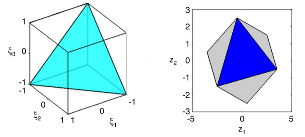
Note that the continuous, original zonotope is in gray.

Notice that the blue region is where

\[{\begin{equation}\left[ \begin{matrix} 1 & 1 & 1 \end{matrix}\right]\xi =-1\end{equation}}\]

(Recall that factors \({\bf\xi}\) lie within the interval \([-1,1]\))

Hybrid zonotopes

Hybrid zonotopes are a superset of constrained zonotopes, which are in turn a superset of standard zonotopes. H-zonotopes allow for constraints like above, but they also add support for binary generators (I’ll get to these).

H-zonotopes take the form:

\[\begin{equation} Z_h=\left\{\bf c+G^c\xi^c+G^b\xi^b \right\}\\ = \{\bf c,G^c,G^b,A^c,A^b,b\}\end{equation}\]

where

\[\begin{equation} {\bf||\xi^c||_\infty} \le1,\\ {\bf |\xi_i^b|}=1 \forall {\bf \xi_i^b\in\xi^b},\\ {\bf A^c\xi^c+A^b\xi^b=b}\end{equation}\]

We call \(Z_h=\{\bf c,G^c,G^b,A^c,A^b,b\}\) the Hybrid Constrained Generator representation (HCG-rep).

Binary generators are used like the continuous generators from standard and constrained zonotopes, but their corresponding weights \(\xi\) can only be \(\pm1\), nothing in between. This means that they effectively translate the corresponding zonotope a distance \(g_i\) from the center \(\bf c\).

Here’s an example of a hybrid zonotope that my labmate Josh showed me:

\[\begin{equation} {\bf c=\left[ \begin{matrix} 0 \\ 0 \end{matrix} \right]} \\ {\bf G^c = \left[ {\begin{matrix} 5 & 5 \\ 5 & 0 \end{matrix}}\right]} {\bf G^b = \left[ {\begin{matrix} 10 \\ 5 \end{matrix}}\right]}\end{equation}\]

This forms a hybrid zonotope as below:

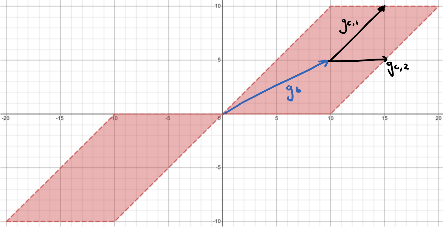
Above: Josh’s example of a hybrid zonotope.

Conclusion

Here I’ve explained four set classes that are each useful in representing and transforming data. I’m especially interested in constrained zonotopes, which can be applied to robot state estimation.

I’ve also introduced some set representations, namely H-rep, V-rep, G-rep, CG-rep, and HCG-rep.

In a future post, I’d like to describe why zonotopes are so useful. To give a hint, constrained zonotopes can be used to model uncertainties in a state estimation problem, and they often offer more flexibility, efficiency, and transparency over alternatives like Gaussian distributions. Adding new information (such as from new sensors or observations) is as simple as appending a generator and/or a constraint.

Appendix

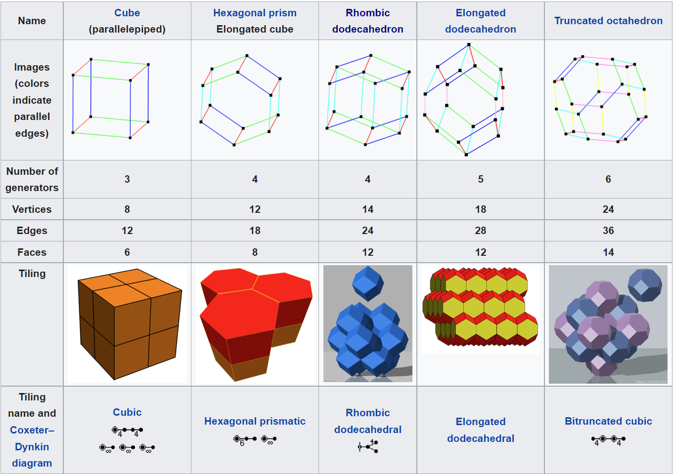
Parallelohedrons

Polytopes that can be translated without rotation to fill a honeycomb space. There are five types: cube, hexagonal prism, rhombic dodecahedron, elongated dodecahedron, and truncated octahedron (Wikipedia).

p-normals

A p-norm is defined as

\[\begin{equation} ||x||_p=[\sum |x_i|^p]^{1/p} \end{equation}\]

Each value of \(p\) forms a unique superellipse (Lamé curve).

When \(p=2\), a Euclidean norm generates a unit ball (e.g. circle for two dimensions).

\(p=1\) results in a diamond shape in two dimensions. \(p=\infty\) forms the infinity norm, which in turn forms the infinity ball (a square in two dimensions). Doesn’t “infinity ball” sound like some sort of fantasy movie prop?

By Quartl - Own work, CC BY-SA 3.0, link

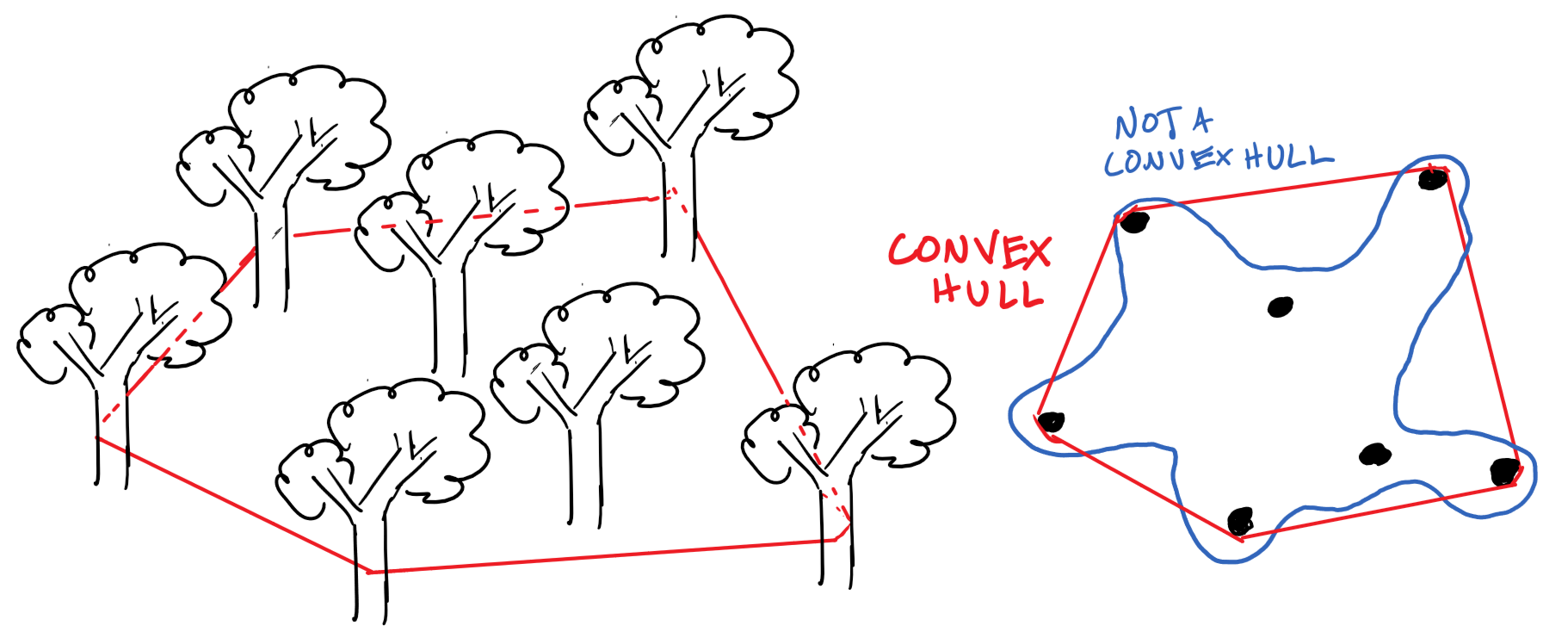
Convex hull

The smallest convex set that fully contains a group of points. Imagine you’re wrapping tape around a grove of trees, taking care to keep the tape tense. A full wrap around the grove forms the convex hull.

Minkowski sum

I just think of this as dragging one set along the perimeter of another set. The area covered by this dragging motion forms a second set, the Minkowski sum. This works just fine with line segments, which form the basis of zonotopes.

Above: Animation of the Minkowski sum of two triangles. Credit: RavenclawPrefect.

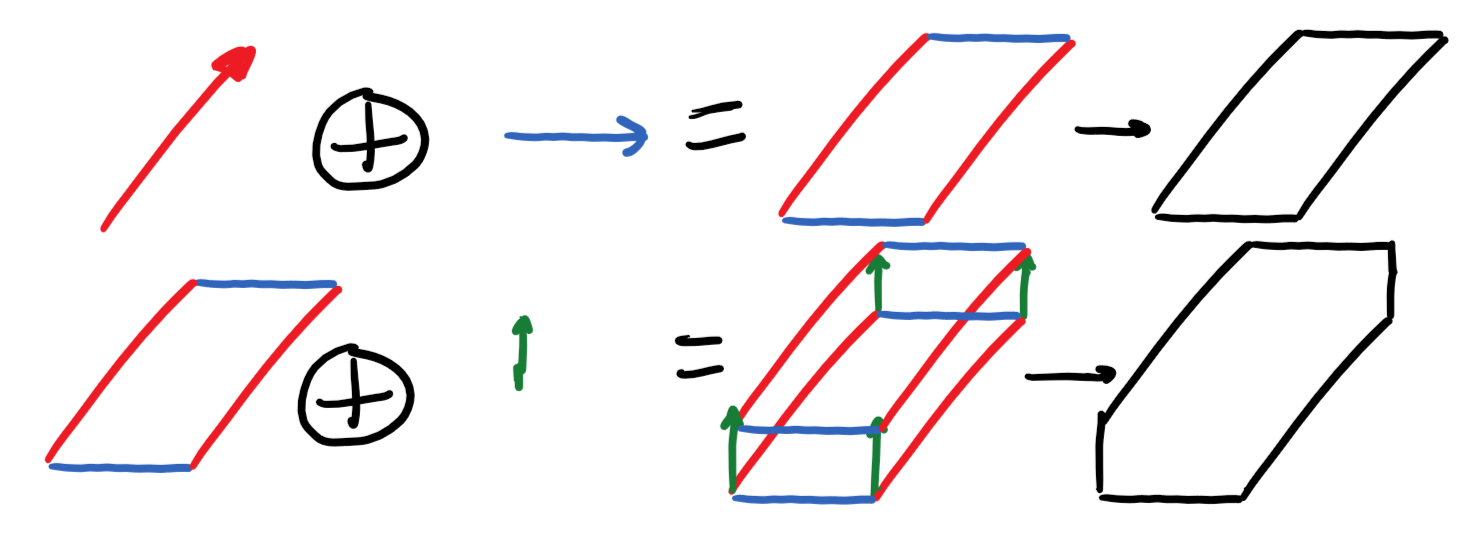
Above: Minkowski sum of two vectors forms a parallelogram. Adding another vector forms a convex hexagon. Both results are also zonotopes by definition!

Acknowledgements

Thank you to Joshua Ortiz for explaining hybrid zonotopes to me. This new form of zonotope was developed in part here at UT Dallas by Dr. Justin Koeln.

Thank you to my research mentor, Dr. Justin Ruths, for exposing me to constrained zonotopes and for showing me their potential.