L1: Foundations of Deep LearningThe perceptronLossTraining neural netsExampleNeural networks in practiceFinding $\eta$ BatchingOverfitting

L1: Foundations of Deep Learning

If we repeat a number of simple mathematical operations millions, billions, even trillions of times, these simple additions, multiplications, and so on begin to develop a complexity seemingly greater than the sum of their parts. Machines that perform enough calculations in just the right structure seem to develop their own personalities, forming "ghosts in the machine."

Machine learning has been around for a long time. Many of the underlying concepts, such as backpropagation and stochastic gradient descent, were established decades ago, but only recently has our technology allowed us to achieve the sheer scale required for the ghosts to emerge.

Let's begin by settling some broad terms. First, AI is a technique that enables computers to mimic human behavior. Within AI, machine learning (ML) is the ability for computers to learn without explicit programming. And within ML, deep learning is the extraction of patterns from data using neural networks.

The perceptron

Neural networks are made of individual units that are sometimes called "nodes," sometimes "neurons," and formally called perceptrons. Each perceptron solves math problems that might appear on a first grader's homework assignment.

$x$ $w$ $\hat{y}$ $\hat{y}=wx$ $w$ is basically just the slope of a line. It turns out that if we were to link all of these perceptrons together, forming a network of perhaps a billion of them, our network's final output would still be linearly related to our input. If our perceptrons simply multiply our input, creating a linear operation, then a network of these perceptrons will only be able to see the world in a linear fashion.

non-linear function $g(z)$ $\hat{x}$ bias $w_0$ $b$ $y=mx+b$ .

Our perceptron's calculation then becomes:

\begin{matrix} (11) & \hat{y} = g (\sum_{i = 1}^{m} x_{i} w_{i}) \end{matrix}

In other words, our perceptron first multiplies each input by its respective weight, sums all of these products together, and sends the result through our non-linear function.

$g(z)$ ? There are many options, including the sigmoid, hyperbolic tangent, and a simple function called the "rectified linear unit," or ReLU.

$\ref{Eq1}$ ) into a matrix operation:

\begin{matrix} (12) & \hat{y} = g (w_{0} + X^{T} W) \end{matrix}

where

\begin{matrix} (13) & \begin{matrix} X = [\begin{matrix} x_{1} \\ ⋮ \\ x_{m} \end{matrix}], W = [\begin{matrix} w_{1} \\ ⋮ \\ w_{m} \end{matrix}] \end{matrix} \end{matrix}

$\hat{y}$ . We call this simple network architecture the sequential model.

Loss

Loss $i$ , loss takes the form

\begin{matrix} (14) & L (f (x^{(i)}, W), y^{(i)}) \end{matrix}

$f(x^{(i)}, W)$ prediction $y^{(i)}$ is the ground truth. Empirical loss is the total loss across an entire dataset:

\begin{matrix} (15) & J (W) = \frac{1}{n} \sum_{i = 1}^{n} L (f (x^{(i)}, W), y^{(i)}) \end{matrix}

Cross entropy loss is used for models that output probabilities (values between 0 and 1):

\begin{matrix} (16) & J (W) = - \frac{1}{n} \sum_{i = 1}^{n} y^{(i)} \log (f (x^{(i)}, W)) + (1 - y^{(i)}) \log (1 - f (x^{(i)}, W)) \end{matrix}

Finally, mean squared error (MSE) is used for regression models with continuous real numbers:

\begin{matrix} (17) & J (W) = \frac{1}{n} \sum_{i = 1}^{n} (y^{(i)} - f (x^{(i)}, W))^{2} \end{matrix}

Training neural nets

$W^*$ $J(W)$ :

\begin{matrix} (18) & W^{*} = \underset{W}{argmin} J (W) \end{matrix}

gradient descent $w_i \in W$ $\frac{\delta J(W)}{\delta w_i}$ . Across all weights, this is equivalent to:

\begin{matrix} (19) & \begin{matrix} \nabla J (w_{1}, w_{2}, \dots, w_{n}) = [\begin{matrix} \frac{\partial J}{\partial w_{1}} (w_{1}, w_{2}, \dots, w_{n}) \\ \frac{\partial J}{\partial w_{2}} (w_{1}, w_{2}, \dots, w_{n}) \\ ⋮ \\ \frac{\partial J}{\partial w_{n}} (w_{1}, w_{2}, \dots, w_{n}) \end{matrix}] \end{matrix} \end{matrix}

$w_i$ increase the cost $J(W)$ $w_i$ learning rate $\eta$ .

Since this process requires us to calculate the partial derivates from the end of the network back to the beginning, we call it backpropagation.

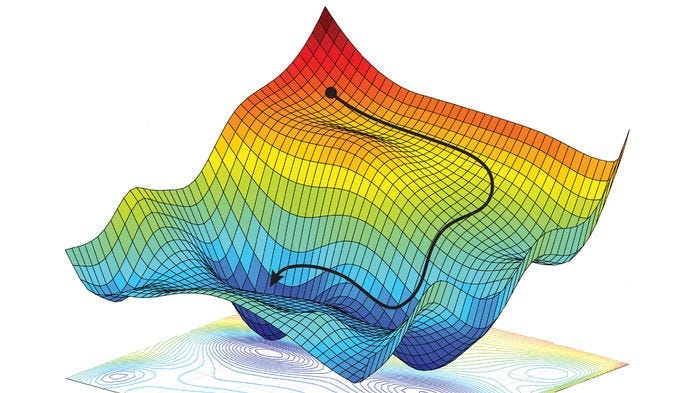
Gradient descent for two variables (3D plot)

Gradient descent across two variables. [Source]

Example

Consider the simplified network above. The partial derivatives via the chain rule are:

\begin{matrix} (20) & \begin{matrix} \frac{δ J (W)}{δ w_{2}} = \frac{δ J (W)}{δ \hat{y}} * \frac{δ \hat{y}}{δ w_{2}} \\ \frac{δ J (W)}{δ w_{1}} = \frac{δ J (W)}{δ \hat{y}} * \frac{δ \hat{y}}{δ z_{1}} * \frac{δ z_{1}}{δ w_{1}} \end{matrix} \end{matrix}

Neural networks in practice

$\eta$

$\eta$ can be tricky. Make it too big, and the gradient descent will skip over the minimum, preventing convergence. Make it too small, and gradient descent will take a long time to converge, in some cases getting stuck in local minima.

$\eta$ by brute force, starting with their best guess and adjusting it. A smarter way would be to use some algorithm to adapt our learning rate during training based on the current characteristics of the network. There are lots of gradient descent algorithms that take this smarter approach, includng:

Stochastic gradient descent
Adam
Adadelta
Adagrad
RMSProp

Batching

Gradient descent is a very expensive calculation to perform. To speed it up, we can run GD on just a selection of our training data. Since this selection should approximately represent the whole dataset, we should achieve similar results while achieving much higher performance.

Overfitting

Overfitting prevents our models from generalizing to new information. We can employ regularization techniques to prevent overfitting. These constrain the optimization problem during training to discourage complex models.

The most popular regularization method is called dropout. In this approach, we randomly select some nodes in our network and set their activations to zero. This random selection, typically about 50% of a network's perceptrons, changes during each training cycle, and prevents the network from relying too heavily on any single node.

Early stopping, a very broad category of regularization, identifies the point of divergence between training and test set accuracies during training. When the two accuracies diverge, this is a clear sign that overfitting has begun.